How Speech Recognition Works: A History From 1952 to Now
Summarize this article with:
Speech recognition converts audio into text by extracting acoustic features from the sound signal and passing them through a model trained to predict words. Today's systems are end-to-end neural networks trained on hundreds of thousands of hours of audio. But that outcome required seven decades of research: from simple pattern matchers in the 1950s, through probabilistic statistical models in the 1980s, to the deep learning revolution of the 2010s that finally made the technology broadly useful.
Speech recognition works by converting a sound wave into a numerical representation of its frequency content, then using a trained model to predict what words were spoken. That one-sentence answer is accurate today, but it obscures seventy years of wrong turns, paradigm shifts, and a few critical breakthroughs that changed what the field thought was possible.
This post traces the full arc, from the first machines that could recognize spoken digits in 1952 to the transformer models that now match human accuracy on clean audio. The engineering internals of today's neural pipeline are covered in our sibling post on how AI speech recognition works, and the product-side pipeline (upload, VAD, diarization, formatting) is in how AI transcription works. This post is the historical foundation both of those build on.
The 1950s: Audrey and a Very Limited Start
Bell Labs' Audrey, built in 1952, is the acknowledged first speech recognition system. It occupied a six-foot relay rack and could recognize spoken digits zero through nine. That sounds modest, but it was a genuine engineering achievement: Audrey worked by analyzing the formants (resonant frequency peaks) of each spoken digit and matching them to stored templates.
The catch: Audrey achieved up to 97 percent accuracy only if the speaker was male, paused at least 350 milliseconds between each digit, and if the machine had been calibrated to that specific speaker's voice. It worked because digit recognition is a closed-set problem with only ten possible answers. Natural speech, with its enormous vocabulary and continuous flow, was an entirely different problem.
A decade later, IBM unveiled Shoebox at the 1962 Seattle World's Fair. It recognized 16 words: the ten digits plus six arithmetic commands like "plus" and "total." The machine could accept a spoken arithmetic problem and hand off the calculation to an adding machine. Still template-matching, still painfully limited.
The 1970s: DARPA, Beam Search, and the 1,000-Word Barrier
The 1970s introduced government money and a harder target. DARPA's Speech Understanding Research (SUR) program, running from 1971 to 1976, funded a small number of research groups to chase a concrete goal: a system that could understand continuous speech over a vocabulary of at least 1,000 words.
Carnegie Mellon's Harpy system, completed in 1976, met that target. Harpy knew 1,011 words and introduced beam search, a decoding strategy that prunes the space of candidate word sequences as it processes audio rather than exhaustively evaluating every possibility. Beam search is still used in modern decoders.
Hearsay, another CMU system from the same period, took a different approach: layered "knowledge sources" that passed hypotheses up from acoustics to phonemes to words to syntax. It was architecturally interesting but fragile, and it lost to Harpy on the benchmark. The lesson, one the field kept relearning, was that elegant structure matters less than finding something that reliably reduces errors.
The 1980s: Hidden Markov Models Change Everything
The real statistical foundation of modern speech recognition came from Hidden Markov Models (HMMs). Lenny Baum developed the underlying mathematics at Princeton in the early 1970s. James and Janet Baker applied HMMs to speech at Carnegie Mellon for their 1974 PhD work, building the Dragon system that would eventually become a commercial product.
HMMs were a conceptual shift from template matching to probabilistic modeling. Rather than storing a fixed fingerprint for each word and measuring distance from it, an HMM models speech as a sequence of hidden states (the phonemes being produced) with observable outputs (the acoustic features measured from the signal). Given observed features, you ask: what sequence of hidden states most probably generated this?
This matters for several reasons. First, the same word sounds slightly different every time you say it. HMMs handle that variation probabilistically rather than requiring rigid agreement with a template. Second, HMMs compose: you can chain phone-level models into word-level models and word-level models into sentence-level models. Third, HMMs can be trained from data rather than hand-engineered, which meant that more data produced better models.
By the late 1980s, HMMs were paired with Gaussian Mixture Models (GMMs) to produce the acoustic model in what became the standard architecture: a GMM-HMM system with a separate n-gram language model that rescored candidate transcripts by how probable the word sequence was in general text.
The 1990s: Commercial Dictation Arrives
The GMM-HMM framework was good enough to build commercial products. Dragon Dictate launched in 1990 at $9,000 with an 80,000-word dictionary. It was discrete speech: you had to pause between words. IBM's ViaVoice (1996) improved usability with speaker-independent models.
Then in 1997, Dragon NaturallySpeaking launched at $150 and supported continuous speech, recognizing roughly 100 words per minute without trained pauses. That was the first system most people could actually use. It still required a speaker-training session to adapt to your voice, and it still struggled with accents, background noise, and domain-specific vocabulary. But it proved that desktop dictation was viable.
My take: the 1990s systems were impressive given the constraints of the time, but they were fragile in a way that made them exhausting to use. If you drifted from a quiet environment or said something outside the expected patterns, accuracy collapsed. The statistical machinery was right; the data and compute were not yet sufficient.
The 2000s: Scale, Neural Nets, and Google's Bet
Google Voice Search, launched in 2008, applied a critical insight: large datasets and distributed computing could produce models that handled accents and noise robustly in a way that no amount of hand-tuning of a small-data system could match. The underlying models were still largely GMM-HMM, but the training data was orders of magnitude larger than what academic researchers had used.
Meanwhile, Geoffrey Hinton and collaborators were demonstrating that deep neural networks could outperform GMMs at acoustic modeling. The landmark 2012 paper "Deep Neural Networks for Acoustic Modeling in Speech Recognition," co-authored by Hinton, Li Deng, Dong Yu, George Dahl, and others from Microsoft, IBM, Google, and Toronto, showed that replacing the GMM with a deep neural network in an otherwise standard HMM pipeline produced large accuracy improvements across multiple benchmarks. The DNN-HMM hybrid cut error rates dramatically on systems that had barely improved for years.
This was not a small incremental step. The field shifted almost immediately. Within a few years, every major commercial ASR system had replaced GMM acoustic models with DNNs.
The 2014-2017 Era: End-to-End Learning
The DNN-HMM hybrid was better, but it was still a three-component system: acoustic model, pronunciation dictionary, language model. Each piece was trained separately and had to mesh at inference time. Researchers started asking whether you could train a single model that mapped audio directly to text.
Two approaches emerged almost simultaneously.
Connectionist Temporal Classification (CTC), introduced by Alex Graves in 2006 but gaining traction in ASR by 2014, provided a way to train sequence-to-sequence models without requiring aligned input-output pairs. Baidu's Deep Speech used a bidirectional RNN with CTC loss to break the Switchboard Hub5'00 benchmark in 2014 without using traditional phoneme dictionaries or hand-engineered features.
Attention-based encoder-decoder models borrowed from machine translation. Work by Chorowski, Bahdanau, and colleagues in 2015 showed that soft attention over the acoustic sequence could replace the explicit alignment enforced by HMMs. The model learned to align on its own.
Both approaches were "end-to-end" in the sense that a single neural network learned everything from data, acoustic patterns and language patterns together, without requiring separate components or pronunciation dictionaries.
2017 and the Transformer
The 2017 paper "Attention Is All You Need" by Vaswani and colleagues at Google introduced the Transformer architecture for sequence modeling. It replaced the recurrent neural networks that had dominated NLP and ASR with self-attention layers that could model relationships between any two positions in a sequence without the sequential bottleneck of RNNs.
Transformers could process the full input sequence in parallel, model long-range dependencies efficiently, and scale up with more data and compute in ways that RNNs struggled to match. By 2019 and 2020, transformer-based ASR systems were reaching state-of-the-art results on standard benchmarks.
Facebook AI's wav2vec 2.0 (2020) demonstrated that transformers could also be pretrained on unlabeled audio in a self-supervised manner, then fine-tuned on small amounts of transcribed data. Training on 53,000 hours of unlabeled audio and fine-tuning on just ten minutes of labeled data produced word error rates that had required thousands of labeled hours under earlier approaches. This was significant for low-resource languages with little transcribed data, a problem covered in detail in our post on why AI struggles with low-resource languages.
2022 to Now: Whisper and the Scale Payoff
OpenAI released Whisper in 2022. The model is a standard encoder-decoder transformer, but its training data was unprecedented in scale and diversity: 680,000 hours of audio paired with transcripts, including 563,000 hours of English and 117,000 hours across 96 other languages, collected from the web.
The audio is converted to an 80-channel log-mel spectrogram computed on 25-millisecond windows at 16,000 Hz before entering the encoder. The decoder generates text tokens autoregressively. Nothing about the architecture is exotic; the scale of the training data is what made the difference.
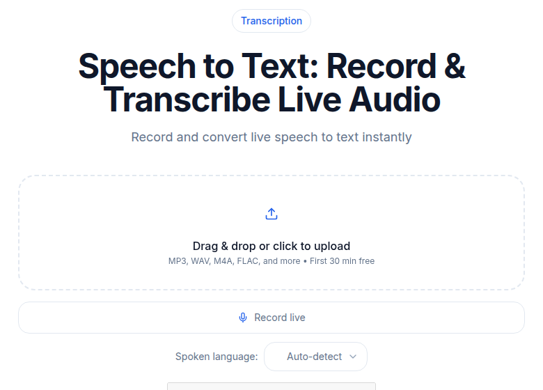 ConvertAudioToText audio upload and transcription tool
Whisper Large-v3 achieves around 3 percent word error rate on clean read speech benchmarks. Real-world accuracy varies significantly with audio quality: on clean recordings it can fall below 5 percent WER, while noisy or conversational audio with multiple speakers can push error rates into the 15 to 30 percent range. For comparison, human transcribers typically achieve 2 to 4 percent WER under good conditions and 10 to 15 percent in noisy environments.
For a ground-level explanation of what WER means and why it can mislead you, see our post on transcription accuracy explained.
Why It Took 70 Years
Three constraints held the field back and each had to be solved roughly in order.
Data. Whisper trained on 680,000 hours. Dragon NaturallySpeaking in 1997 trained on far less, and the models it could learn were correspondingly shallower. Collecting and labeling audio at scale was expensive; the web eventually provided it for free.
Compute. Training a transformer on 680,000 hours requires GPU clusters. The 2012 DNN-HMM breakthrough coincided with the GPU computing era becoming accessible enough to run deep networks on research budgets. Earlier, the compute simply was not available.
Algorithms. HMMs were the right framework for the data and compute available in the 1980s. Deep nets were theoretically compelling earlier but practically untrainable on the hardware and dataset sizes that existed. Transformers solved the parallelism and long-range dependency problems that made RNNs hard to train at scale.
The lesson: each generation of researchers was working near the frontier of what their constraints allowed. The 1952 Audrey team did something genuinely hard with template matching and analog circuits. The 1980s HMM work was statistically rigorous and durable. The 2012 deep learning pivot was fast precisely because the ideas had matured and the compute had caught up. Understanding that progression makes the current transformer era look less like magic and more like the next iteration of the same pattern.
If you want to see modern end-to-end recognition in practice, the audio-to-text tool at ConvertAudioToText runs files through the current pipeline, and the output you get back is the product of everything described above.
FAQ
What was the first speech recognition system?
Bell Labs built Audrey in 1952. It could recognize the digits zero through nine, but only from a single speaker under controlled conditions. It occupied a six-foot relay rack and worked by matching the formant frequencies of each digit to stored templates.
What are Hidden Markov Models and why did they matter for speech recognition?
Hidden Markov Models (HMMs) model speech as a sequence of hidden states (phonemes) that produce observable outputs (acoustic features). Rather than matching audio to a fixed template, HMMs compute the most probable sequence of phonemes that could have generated the observed audio. This probabilistic framing handled natural variation in pronunciation and scaled to large vocabularies in a way that earlier template-matching approaches could not.
What changed in 2012 to make speech recognition so much better?
The 2012 breakthrough was replacing the Gaussian Mixture Model (GMM) acoustic component in the standard GMM-HMM pipeline with a deep neural network. A paper by Hinton, Deng, Yu, Dahl, and collaborators from Microsoft, Google, IBM, and the University of Toronto demonstrated that DNN-HMM hybrid systems substantially outperformed GMM-HMM baselines on multiple benchmarks, triggering rapid adoption across the industry.
What does "end-to-end" mean in speech recognition?
An end-to-end system is a single neural network trained to map audio directly to text, without separate acoustic models, pronunciation dictionaries, or language models that have to be trained and combined separately. Baidu's Deep Speech (2014) was an early high-profile example using CTC loss. Whisper is a more recent example using an encoder-decoder transformer architecture. The main advantages are simpler training pipelines and the ability to optimize everything jointly toward the final transcript.
How accurate is modern speech recognition?
On clean, well-recorded single-speaker audio, state-of-the-art models reach below 5 percent word error rate (WER). On noisy, conversational, or multi-speaker audio, WER commonly falls in the 15 to 30 percent range. Human transcribers achieve roughly 2 to 4 percent WER under good conditions and degrade to 10 to 15 percent in difficult audio. Accuracy depends most on audio quality: background noise, overlapping speakers, and low recording bitrate are the main factors that push error rates up even with the best models.
Sources
- OpenAI Whisper announcement and technical details: https://openai.com/index/whisper/
- Whisper technical paper via OpenWhispr summary: https://openwhispr.com/blog/how-whisper-ai-works
- History of speech recognition milestones (Milvus): https://milvus.io/ai-quick-reference/what-is-the-history-of-speech-recognition-technology
- History of ASR (Descript/Medium): https://medium.com/descript/a-brief-history-of-asr-automatic-speech-recognition-b8f338d4c0e5
- Audrey and early systems, Computer History Museum: https://computerhistory.org/blog/audrey-alexa-hal-and-more/
- Janet M. Baker Wikipedia (HMM/Dragon origins): https://en.wikipedia.org/wiki/Janet_M._Baker
- James K. Baker Wikipedia: https://en.wikipedia.org/wiki/James_K._Baker
- 2012 DNN-HMM paper (Hinton et al.), IEEE Signal Processing Magazine: https://www.cs.toronto.edu/~gdahl/papers/deepSpeechReviewSPM2012.pdf
- CTC, Wikipedia: https://en.wikipedia.org/wiki/Connectionist_temporal_classification
- wav2vec 2.0 paper (arXiv): https://arxiv.org/pdf/2006.11477
- "Attention Is All You Need" (arXiv): https://arxiv.org/abs/1706.03762
- WER benchmarks and accuracy discussion (AssemblyAI): https://www.assemblyai.com/blog/word-error-rate-is-broken
- DARPA SUR program and Harpy (CMU historical document): https://rr.cs.cmu.edu/SUR.pdf
- Sampling rate and Nyquist for ASR (Picovoice): https://picovoice.ai/blog/audio-sampling-and-sample-rate/
Try transcription free
Convert any audio or video to clean, unwatermarked text — speaker labels, timestamps, and AI summaries included. First 30 minutes free, no account.
Related Articles

Acoustic Models vs Language Models in Speech Recognition
What acoustic models and language models do in ASR, why the split mattered historically, how end-to-end systems absorbed it, and why it still explains the errors you see today.
Neural Networks and Transcription: How Models Learn to Listen
A plain-language guide to how neural networks convert speech to text: features, layers, transformers, training data, and where modern ASR still fails.