Neural Networks and Transcription: How Models Learn to Listen
Summarize this article with:
Modern transcription accuracy comes almost entirely from neural networks trained on millions of hours of audio. A speech model is a stack of mathematical functions that learns acoustic patterns in its early layers, phonetic structure in its middle layers, and language context in its late layers. The transformer architecture, introduced in 2017, replaced older recurrent networks and allowed models to handle long-range dependencies in audio directly. Whisper Large-v3, for example, trained on roughly 5 million hours of audio and uses 128 mel-frequency channels as input.
Modern transcription accuracy is built on neural networks. The gains between 2015 and today came almost entirely from better architectures and larger training sets, not from clever hand-crafted rules layered on top. This post maps the core neural network concepts to what actually happens inside a transcription model.
What a Neural Network Is, at the Minimum Useful Level
A neural network is a stack of mathematical functions with many adjustable parameters. You train it by showing it millions of input-output pairs, adjusting the parameters each time the network produces the wrong output. After enough training, the network generalizes: it produces correct outputs for inputs it has never seen.
For speech recognition, the inputs are audio representations and the outputs are text tokens. That is the whole framework. The interesting questions are about the shape of the input, what the different layers actually learn, and why training data determines the ceiling on accuracy.
What the Network Sees as Input
Modern speech recognition networks do not operate on raw audio samples. They operate on spectrograms: 2D images that show how frequency energy is distributed over time.
Whisper Large-v3 takes a log-mel spectrogram with 128 frequency channels as input, one frame every 10 milliseconds. This is a deliberate increase from the 80 channels used in earlier Whisper versions. The upgrade gives the model finer-grained frequency resolution, which helps particularly with tonal languages and closely spaced vowels.
Our post on how speech recognition works covers the spectrogram conversion in more detail. For this post, the key point is that the network sees something like a photograph of the audio, not the audio itself.
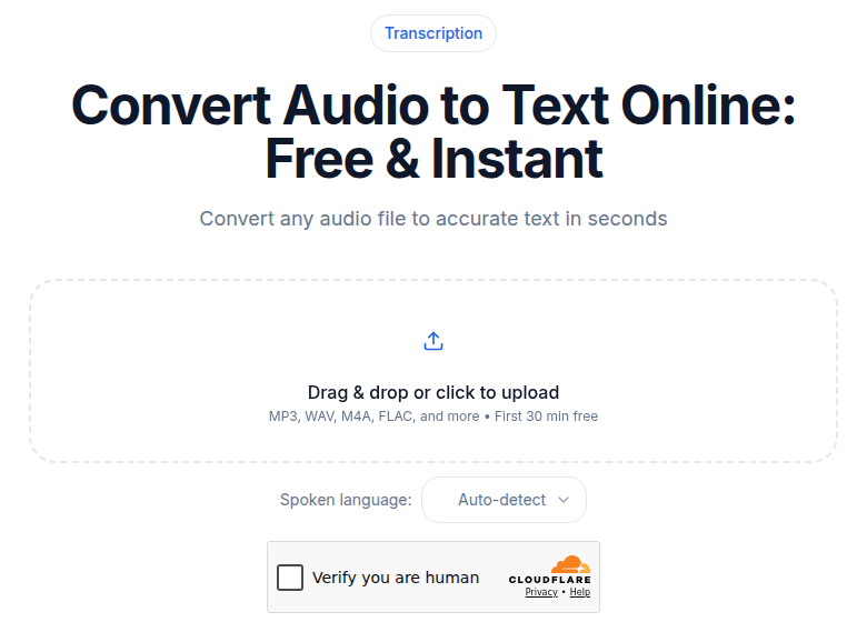 The audio upload interface at ConvertAudioToText, where uploaded files are converted to spectrograms before transcription
Layer by Layer: What the Model Learns
Deep neural networks develop internal representations that become progressively more abstract as you move from the first layer to the last. For speech recognition, the pattern follows a rough three-stage hierarchy.
Early Layers: Acoustic Features
The first few layers detect low-level acoustic patterns. A voiced consonant has a different spectral signature than an unvoiced one; a vowel differs from a fricative. These distinctions map roughly onto the distinctions a phonetician would draw, though the model was never told to look for them explicitly.
Research mapping Whisper's internal representations to human neural data shows that early layers correlate most strongly with onset-related acoustic processing, which is consistent with what we know about early auditory cortex.
Middle Layers: Phonetic and Syllabic Patterns
Middle layers combine low-level features into higher-level units: phonemes, syllables, short word fragments. By this stage, the network has compressed the raw acoustic signal into a representation that captures linguistic content while discarding speaker-specific details like pitch and vocal tract size.
This is also where the model learns to be invariant to things that should not affect the transcript: recording quality, accent variation, background noise (within limits). The model does not explicitly learn any of this; the training signal is simply "produce the right text," so the model discovers invariances that help it do so. Our post on acoustic models versus language models covers the historical division of these jobs between separate systems.
Late Layers: Linguistic Context
Late layers in the encoder and the decoder layers are where language modeling happens. The model learns that certain word sequences are more probable than others, that grammatical constructions are common and ungrammatical ones are not, and that particular words tend to appear in particular contexts.
This is what allows the model to resolve acoustically ambiguous phrases. The phrase "recognize speech" sounds nearly identical to "wreck a nice beach" when spoken quickly. The language modeling capacity picks the right interpretation based on surrounding context. The example has been a running joke in the field since the 1960s, when engineer Manfred Schroeder discovered his vocoder kept rendering his test phrase that way.
The Transformer Architecture
Almost every competitive speech recognition model today uses a transformer. The architecture was introduced in 2017 in the paper "Attention Is All You Need" (Vaswani et al.) for machine translation. It turned out to generalize well to almost every sequence modeling task, including speech.
The core mechanism is self-attention. Each position in the input sequence gets to attend to every other position, with learned weights that determine how much each position "cares about" each other. For audio, this means a word at second 12 can directly use context from second 4 without needing to propagate information through every intermediate step.
Older recurrent networks (RNNs and LSTMs) processed sequences one step at a time and struggled to retain information across long gaps. Transformers handle long-range dependencies more naturally, which matters because the correct interpretation of a word in a transcript often depends on context from many seconds earlier.
Encoder-Decoder Structure
For speech recognition, the standard transformer arrangement is encoder-decoder. The encoder reads the full spectrogram and produces a sequence of high-dimensional vectors, one per time frame. The decoder then generates text tokens one at a time, attending to the encoder output at each step.
Whisper Large-v3 uses this structure. So do most competitive open-source speech recognition models. Our post on Whisper Large-v3 explained covers the specific architecture in more detail.
How Training Actually Works
You start with random parameters. The model produces nonsense. You compute the error between the model's output and the correct transcript, propagate that error backward through the network (backpropagation), and adjust each parameter slightly in the direction that reduces the error. Repeat this process billions of times across millions of training examples.
The mechanics involve batches (many examples at once for efficiency), learning rate schedules (how aggressively you update parameters over time), and regularization techniques to prevent overfitting. For a model the size of Whisper Large-v3, training runs for days to weeks on hundreds of GPUs.
Why Training Data Determines the Ceiling
The model can only learn patterns that exist in its training data. If the training data is all studio-recorded English, the model will underperform on telephone audio or non-native speakers. If the training set has no medical vocabulary, the model will misspell drug names.
Whisper Large-v3 trained on approximately 5 million hours of audio total: roughly 1 million hours of weakly labeled audio and an additional 4 million hours of pseudo-labeled audio generated by running Whisper Large-v2 over unlabeled content. This is significantly more than the 680,000 hours used to train the original Whisper release.
Deepgram Nova-3, released in early 2025, trained on a proprietary dataset spanning over 100 domains and tens of billions of tokens. The scale and domain diversity of training data is one of the main reasons models from well-resourced labs outperform smaller alternatives in real-world conditions.
Fine-tuning is the practical solution when a general model underperforms on your domain. You take a pretrained model and continue training on a small amount of domain-specific data: a few hours of medical recordings, legal depositions, or technical podcasts. Because the model already knows language and acoustic structure, it only needs to adjust the parameters that matter for your vocabulary. See our post on transcription accuracy explained for more on how domain mismatch shows up in error rates.
What Happens at Inference Time
Once trained, using the model is straightforward. You provide audio, the model produces text.
The inference process:
- Audio is converted to a log-mel spectrogram.
- The encoder processes the spectrogram and produces a sequence of hidden vectors.
- The decoder generates text tokens one at a time, conditioning each new token on the encoder output and all previously generated tokens.
- Generation stops when the decoder produces an end-of-sequence token.
For a 30-second clip, this takes a fraction of a second on modern hardware. Longer audio is processed in 30-second chunks and stitched together.
Why End-to-End Beat Hybrid Systems
Before roughly 2017, speech recognition systems were hybrid: a neural network estimated phoneme probabilities, a pronunciation dictionary mapped phonemes to words, a separate language model scored word sequences, and a beam-search algorithm combined everything.
End-to-end systems collapsed all of this into a single network trained directly on audio-to-text pairs. The training objective is simply "produce the right text from the audio," and the model learns whatever internal structure serves that goal.
Three concrete reasons this works better:
The model can use information the hybrid designers did not anticipate. Prosodic features like intonation, stress, and rhythm can disambiguate words that sound identical in isolation. Hybrid systems rarely used prosody; end-to-end models pick it up incidentally during training.
Joint optimization is more efficient than tuning separate components. A hybrid system is limited by its weakest module. An end-to-end model can learn to compensate for weaknesses in one part with strengths in another.
Transfer across languages is natural. A single Whisper model handles 99 languages because shared internal representations help with all of them. Hybrid systems needed largely separate components for each language.
For more on the architecture choices, see our post on how AI speech recognition works, which covers the encoder-decoder and CTC families in technical depth.
Where Neural Networks Still Fail
Neural networks are not magic. They have systematic failure modes that come directly from the training process.
Long-tail vocabulary. Words that appeared rarely in training data get misspelled consistently: brand names, technical jargon, unusual proper nouns. The model assigns low probability to rare tokens because they seldom appeared in correct transcripts during training. Our post on why transcription makes mistakes covers this in detail.
Distribution shift. Audio that differs significantly from the training distribution, whether due to unusual recording conditions, heavy accent, or novel domain vocabulary, produces worse output. This is not a bug; it is a direct consequence of how training works.
Hallucination. The decoder can produce plausible-sounding text that does not correspond to anything in the audio, particularly during silence or background noise. The model has a strong prior toward producing text because its training data almost always contained speech. Voice activity detection (VAD), which filters out non-speech segments before they reach the transcription model, is the standard mitigation. Our post on how VAD works explains the technique.
Speaker confusion. Standard transcription models produce one undifferentiated stream of text. Separating speakers requires an additional step called diarization. Our post on speaker diarization explained covers how that works separately from the base transcription.
My take: the failure modes listed above all have known mitigations, and the best production systems apply several of them in combination. But understanding the root cause of each failure mode is what tells you which mitigation to reach for, and when it will not help.
A Note on the Product Pipeline
This post focuses on the neural network itself. If you want to understand how the full product pipeline works from upload to formatted transcript, covering VAD, diarization, punctuation restoration, and output formatting, see our post on how AI transcription works. The two posts are meant to be read together.
If you want to try the output of a production neural transcription system on your own audio, ConvertAudioToText transcribes uploaded files with no signup required for short clips.
Sources
- OpenAI Whisper Large-v3 model card: https://huggingface.co/openai/whisper-large-v3
- Vaswani et al., "Attention Is All You Need" (2017): https://arxiv.org/abs/1706.03762
- Deepgram Nova-3 announcement: https://deepgram.com/learn/introducing-nova-3-speech-to-text-api
- WhisperX: Time-Accurate Speech Transcription of Long-Form Audio: https://arxiv.org/pdf/2303.00747
- Calm-Whisper: Reduce Whisper Hallucination On Non-Speech: https://arxiv.org/html/2505.12969v1
- Language Log on "Wreck a Nice Beach": https://languagelog.ldc.upenn.edu/nll/?p=13828
FAQ
What input does a neural network actually receive from audio?
It receives a spectrogram, not raw waveform samples. For most modern models, that means a log-mel spectrogram: a 2D representation of how frequency energy is distributed over time. Whisper Large-v3 uses 128 mel-frequency channels per time frame, an upgrade from the 80 channels used in earlier Whisper versions.
Why did end-to-end neural networks replace hybrid ASR systems?
Older hybrid systems had separate components: a neural network for phoneme probabilities, a pronunciation dictionary, a language model, and a beam-search decoder. Each had to be tuned independently. End-to-end models collapsed all of this into one network trained directly on audio-to-text pairs. The joint training lets the model learn compensating strategies that separate components cannot, and a single Whisper model can serve 99 languages because it shares internal representations across all of them.
Why does a transcription model sometimes produce text that was never said?
This is hallucination: the decoder generates plausible text even when the audio contains only silence, background noise, or unintelligible sound. The model learned from audio that almost always contains speech, so it has a strong prior toward producing text. Voice activity detection (VAD) mitigates this by filtering out non-speech segments before they reach the transcription model.
What is fine-tuning and when does it help?
Fine-tuning means taking a trained general-purpose model and continuing training on a small dataset from a specific domain, such as medical recordings or legal depositions. Because the model already knows language and acoustic structure, it only needs a few hours of domain-specific audio to bias toward correct vocabulary and phrasing. Fine-tuning is most useful for technical vocabulary that appeared rarely in the original training data.
Try transcription free
Convert any audio or video to clean, unwatermarked text — speaker labels, timestamps, and AI summaries included. First 30 minutes free, no account.
Related Articles
How Speech Recognition Works: A History From 1952 to Now
From Bell Labs' Audrey to transformer-based neural networks, this foundational guide traces how speech recognition evolved from digit recognizers to near-human accuracy over 70 years.
How to Transcribe Voice Recorder Recordings (Any Device)
Get text from any voice recorder, from Anker SoundCore Work to old Olympus dictaphones. Covers file transfer, formats, WMA conversion, speaker labels, and export options.